In this post, we’ll go over the basics of deep learning in a concise form, avoiding tricky math when possible. If you don’t understand deep learning already, hopefully by the end of this post you’ll get a gist of how this technology works.
Deep learning is a special kind of machine learning. Simple machine learning algorithms – as opposed to deep learning – are absolutely dependant on how the data has been represented. So, what do I mean by that?
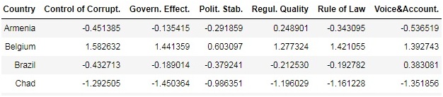
In data science, one of the cornerstone concepts is a feature. A feature is an attribute or property shared by all of the data points in a dataset.
For example, in this table, each country represents a data point, and each column (‘Control of Corrupt.’, ‘Govern. Effect.’, etc) represents a feature:
Oftentimes, choosing right features is crucially important in order to successfully work with simple machine learning algorithms. Moreover, features have to be manually constructed in the first place, which is, of course, a lot of work to do.
However, deep learning allows constructing features automatically. This is one of the main advantages of deep learning over simple machine learning algorithms. In particular, it allows us to work with more complex problems like image recognition, for example. It also allows us to take advantage of bigger amounts of data (if they’re out there).
Though, the quality of data is extremely important for successful work with deep learning too.
The critical property of deep learning
At the heart of deep learning lies the process of building complex functions out of simpler ones.
In mathematics, a function is simply a rule that matches some inputs to some outputs. Note, if we know a sufficient quantity of input-output matches, we can infer or learn a corresponding rule or a function.
For example, from a given set of input-output matches:
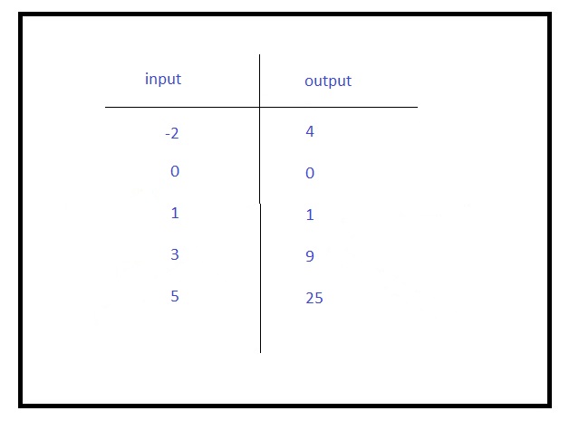
we can infer that this function most likely squares the input. Of course, the more instances of input-output correspondence we have, there more reliable is our inference.
Sometimes functions are very simple, like in the previous example, but sometimes not.
Many functions have multiple variables, for example:
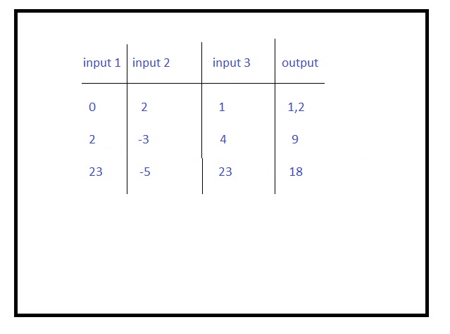
It’s probably more difficult to learn this function than the previous one. (Moreover, in deep learning tasks, we need to find minimums of functions)
Note that every process in the universe can be viewed as a function.
For example, the work of the brain is a function. The brain receives the input from the sensory organs and sends signals to the rest of our body. This is an extraordinary complex multidimensional function. By the way, if someday machines learn this function and are able to implement it, we would have artificial general intelligence.
Any complex continuous function can be broken down into a finite set of smaller components (functions of one variable). By the way, this theorem was first proved by the famous mathematician Andrey Kolmogorov back in the 1950s.
Apparently, learning complex functions becomes much easier when we can first learn their constituent components. And this process, as we said, is the crux of deep learning. Simple machine learning algorithms aren’t capable of doing this.
In principle, deep learning can be implemented in many ways. But in practice, deep learning is implemented by utilizing so-called deep neural networks.
Perceptrons
Artificial neural networks have been known since the 1950s. First artificial neural networks were perceptrons. As a matter of fact, they’re still in use.
Perceptrons don’t belong to deep neural networks. So, we won’t discuss them in detail in this tutorial.
But we should briefly mention here their capabilities and limitations.
When doing such tasks as classification, perceptrons can separate data points only linearly (by a straight line), that is they implement linear functions. Sometimes it works:
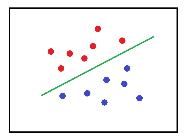
But in many cases, this linear approach totally fails. For instance, like in this example, where we can’t separate blue and red circulars by drawing a straight line between them:
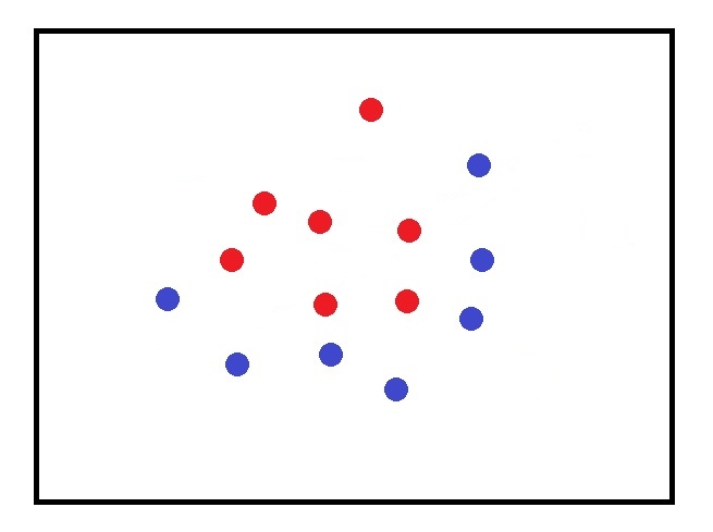
This fact tremendously limits the capabilities of perceptrons.
How artificial neural networks organized
Artificial neural networks like their biological counterparts consist of neurons or nodes which are grouped in layers.
There are three basic types of layers: input, output, and hidden.
The input layer only receives information. The hidden layers perform some calculations. The output layer also performs some calculations and gives us new information, which usually represents a solution to a certain problem.
If we have only one hidden layer (perceptrons don’t have one), formally speaking, our neural network is deep. But in practice, deep learning usually refers to networks with several hidden layers and more.
Let’s take a peek how an artificial neuron works.
A neuron receives some inputs that are multiplied by weights. Then we add these products to each other and also usually add another component called bias.
(A neural network has an ability to adjust its weights and biases during training. We’ll get to that shortly.)
Then we throw this sum in a nonlinear function called activation function.
There are many activations functions in use. For example, a very common one is so-called ReLU (Rectified liner unit) function.
As depicted, ReLU just turns all not positive values to zero. Indeed, it’s very simple to compute.
So, now we have a value of our neuron. This value propagates to the neurons in the subsequent layer.
So, the neurons of one layer of a network provide inputs for the neurons in the following layer.
How artificial neural networks learn
But how do neuron networks learn?
Here I should say that there are several types of machine learnings:
Supervised
Unsupervised
Semi-supervised
Reinforcement
The most common type of learning (at least to these days) is supervised learning. In this type of learning, we have labeled data that we give to an algorithm to train on. In this post, I explain how neural networks learn in a supervised way. But almost all of it is also relevant to other types of learning. (Maybe I’ll write a post on unsupervised learning shortly).
The training of a neural network in a supervised way can be described as follows.
Let’s suppose that our task is an image classification and we have two classes: planes and cars. Our dataset consists of images of 50X50 pixel images.
So, our input layer consists of 2500 neurons (because 50X50=2500) in which we can place one image as a single vector.
Also, we have a couple of hidden layers. The output layer has only two neurons since we have only two classes.
As we’re training our network, we give it labeled images of cars and planes.
Each time our network is given a plane its output must be close to 1, and each time the net is given a car its output must be close to 0.
The weights and biases are generated randomly between -1 and 1. After feeding the network with all the training data, if the actual outputs match perfectly with the desired ones (which is extremely unlikely), we finish training. But if it’s not the case, the network should adjust all its weights and biases in such a way that the actual outputs will correspond to the desired ones.
A neural network implements a function with different names: loss, cost, or objective function. In this tutorial, I’ll only use the term “cost function” in order to avoid any ambiguity.
A cost function shows how the actual outputs differ from the correct outputs during the training of a network. A cost function measures how well we are doing on an entire training dataset.
Actually, the learning of a neural network is nothing more than minimizing a cost function.
There are many different cost functions, which can be more or less suitable depending on a task.
And please also don’t confuse a cost function with an activation function. Remember a cost function is implemented by an entire network. Whereas, an activation function is implemented inside an individual neuron.
Gradient-based optimization
In principle, there are many ways to minimize a cost function. But in neural networks, the best method is a so-called gradient-based optimization in conjunction with an algorithm called back-propagation.
The famous algorithms back-propagation or just backprop finds derivatives for every weight and bias in a network. In calculus, a derivative is a measure in which direction and how fast a function is changing at a given point. (A function can increase or decrease.)
Note when dealing with multivariable functions, we actually compute gradients, not derivatives. A gradient is an equivalent of a derivative for multivariable functions. But for the sake of simplicity, you can justifiably imagine a function with one variable as a cost function and use derivatives in order to find its minimum. I always do so.
As a result of backprop, we know whether the function is increasing or decreasing with respect to all weights and biases in a network.
After implementing backprop, a neural network implements gradient-based optimization. In most cases, the algorithm for doing this in deep neural networks is Stochastic Gradient Descent (SGD).
SGD takes iterative steps toward the minimum of a cost function until it reaches this minimum. In SGD – as well as in other types of gradient-based optimization – we should specify the size of our step toward the minimum of a function. In neural networks, this parameter is called a learning rate. Not surprisingly, choosing an appropriate value for a learning rate is important.
In SGD, a cost function is calculated not on entire training dataset at one time but iteratively on its single training example which is taken randomly from the dataset.
There is also Mini-batch gradient descent, where a cost function is calculated iteratively on a certain fraction of a dataset. This fraction is called a batch or mini-batch. Choosing the reasonable number for a batch size pretty much depends on how powerful our hardware is. The more powerful hardware, the greater a batch size can be.
For example, our training dataset consists of 100.000 images, and a batch size is say 100. So, in this case, we should implement 100.000/100=1000 iterations until all the data points are given to the network.
Validating and testing
Having trained a network, we should validate this network on other data. So, in addition to a training set, we should have a validation set. It may be possible that our network works perfectly on a training set but poorly on a validation set. Most likely it happens because of the process called overfitting.
Overfitting occurs when a machine learning algorithm just remembers training data points by heart, but cannot generalize on new data. There are a number of techniques for avoiding overfitting in deep neural networks.
After successful validation, however, we should test a neural network on unlabeled data. So, we should have one more dataset for doing this – a testing dataset. If a network works great on a testing dataset, it can be finally used in production.
I hope, you can benefit from this concise tutorial, where I tried to lay out the basics of deep learning as easy as possible.
References
http://www.deeplearningbook.org/contents/intro.html
http://introtodeeplearning.com/materials/2018_6S191_Lecture1.pdf
http://neuralnetworksanddeeplearning.com