There’ve been proposed several types of ANNs with numerous different implementations for clustering tasks. Most of these neural networks apply so-called competitive learning rather than error-correction learning as most other types of neural networks do. ANNs used for clustering do not utilize the gradient descent algorithm.
Probably, the most popular type of neural nets used for clustering is called a Kohonen network, named after a prominent Finnish researcher Teuvo Kohonen.
There are many different types of Kohonen networks. These neural networks are very different from most types of neural networks used for supervised tasks. Kohonen networks consist of only two layers.
The structure of a typical Kohonen neural network is shown below:
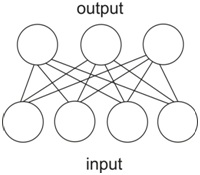
As we see, the network consists of two layers: the input layer with four neurons and the output layers with three layers. If you are familiar with neural networks, this structure may look to you like a very simple perceptron. However, this network works in a different way than perceptrons or any other networks for supervised learning.
We will be working with a famous Iris data set, which consists of 150 samples divided into three classes. The data in the dataset must be normalized.
In our neural network, the number of output neurons is equal to the number of clusters or classes (in our case it is three). However, we can construct a more advanced Kohonen network for dealing with problems where we don’t know the number of clusters beforehand.
In a Kohonen net, each neuron of an output layer holds a vector whose dimensionality equals the number of neurons in the input layer (in our case it is four). In turn, the number of neurons in the input layer must be equal to the dimensionality of data points given to the network. We will be working with a four-dimensional data set. That is why our network has four neurons in its input layer.
Let’s define the vectors of the output layer in our network as w1, w2, w3. These vectors are randomly initialized in a certain range of values.
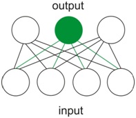
When the network gets an input, the input is traversed into only one neuron of the output layer, whose value is closer to the input vector than the values of the other two output neurons. This neuron is called a winning neuron or the best matching unit (BMU). This is a very important distinction from many other types of neural networks, in which values propagate to all neurons in a succeeding layer. And this process constitutes the principle of competitive learning:
Let’s define the input vectors as x1, x2 … xn, where n is the number of samples in the training set. In our case, n is 150.
After receiving an input vector x, the winning neuron modifies the value of its previous vector w in a loop according to the formula wn = wn+λ (xn-wn), where λ is a coefficient, which we reduce by Δλ in each iteration of the loop unless λ>0. We do this for each x in our training set. We can pick input vectors randomly or in a specific order. In this loop, λ and Δλ are our parameters, which we define and can modify.
As a result of this algorithm, we have a set of w vectors with new values. So, now our network is trained, and we can start clustering. This is a very simple task: for each vector x we find the closest vector w in our trained neural network. Our x vectors can be even not from our dataset we have worked with. If so, such vectors first have to be normalized.
Now, let’s code this network in Python.
First, we import all the packages we need for this task. We only need Numpy and Pandas
Then we download the iris dataset we will work with and show its first five samples in a data frame:
We normalize the data and throw them in a numpy array:
Then, we initiate the number of classes or clusters, the list for the w vectors, the number of the x vectors, and the dimensionality of the x vectors:
Then, we create a function for obtaining random values for the x vectors (or weights), and then we initialize these x vectors:
We create a function for computing the Euclidian distance between our x and w vectors:
We create a function for finding the closest x vectors to the w vectors:
Then, we initialize the λ and Δλ coefficients and start looping to find the closest x vectors to the w vectors:
So, now our network is trained. Finally, we can compare the results of our classification with the actual values from the data frame:
We see that the class “2” completely overlaps with the class ‘Iris-setosa’, the class “1” mostly overlaps with the class ‘Iris-versicolor‘, and the class “0” mostly overlaps with ‘Iris-virginica‘. There are 18 mismatches between ‘Iris-virginica‘ and ‘Iris-versicolor‘ classes, corresponding to 12% of the entire data set. So, the overall correspondence of our results to the actual data is 88%.
Since we initialized the classes “0”, “1”, “2” randomly, the order of these classes can be different in other iterations of this program, but it does not change the structure of the classification.
This code of this network for clustering or unlabeled classification is on my GitHub: https://github.com/ArtemKovera/clust/blob/master/Kohonen%2Bnetwork%2B.ipynb